
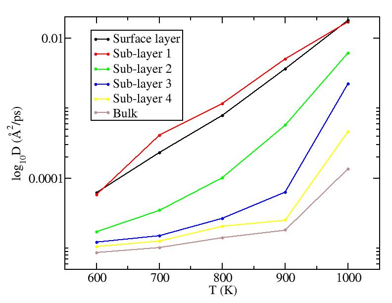
We should add to this graph results from new simulations at 850K, 950K, 1050K and 1075K that Yanting is doing.
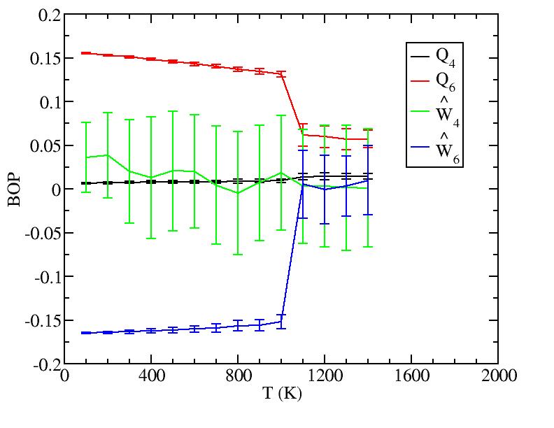
We should add to this graph results from new simulations at 850K, 950K, 1050K and 1075K that Yanting is doing.
Observations: For T=1100K above melting, we see saturation of diffusion for all layers - everyone moves around a lot! For T less than melting, we see primarily diffusion of surface and 1st sublayer. At the higher T, there is some diffusion of the lower sublayers. But the diffusion of sublayers is most likely due to the following effect: atoms only diffuse on surface; sublayer atoms diffuse only because they can get excited up to the surface and start diffusing from there (see figure in next section) - recall, we give each atom its layer number at the start of the simulation at each T, and do not relabel even if atoms move from one layer to another.
It is still odd to me that the 1st sublayer is diffusing more than the surface layer. Any idea why this is so? Is it possibly a misslabeling of the graphs?
Perhaps we should include here curves from the new simulations at T=950, 1050, 1075, depending on how they look.
Should we be concerned about the "glitches" in the data near 800ps? I recall we talked about his earlier, but I forget the reason for the glitch.
Do I recall correctly, that the average spacing between atoms is about 3.6 angstrom? So to set the scale of these graphs, a MSD of about 13 corresponds to diffusing one inter-atomic spacing?
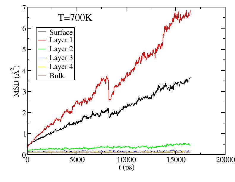
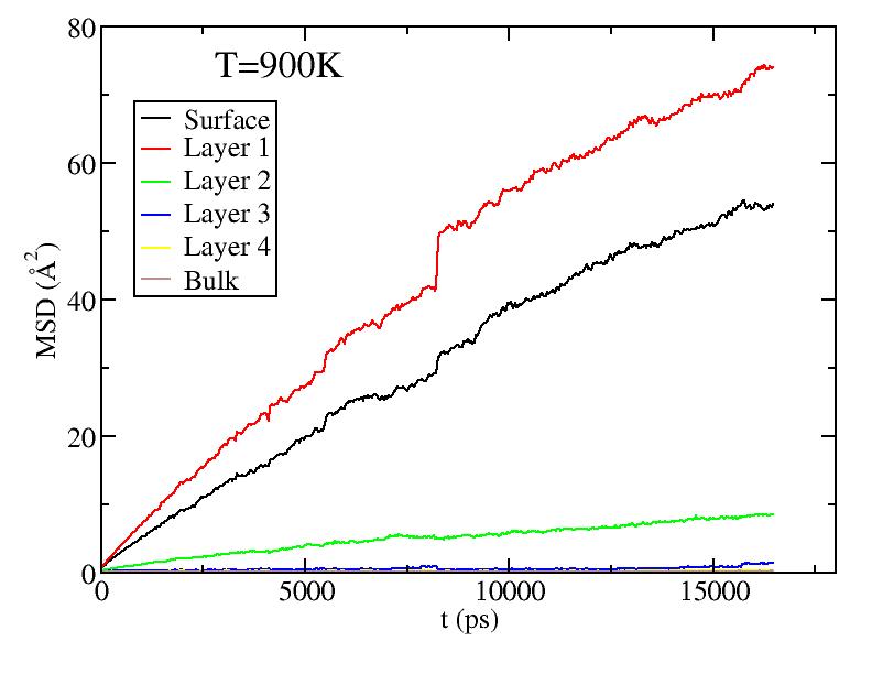
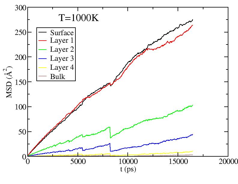
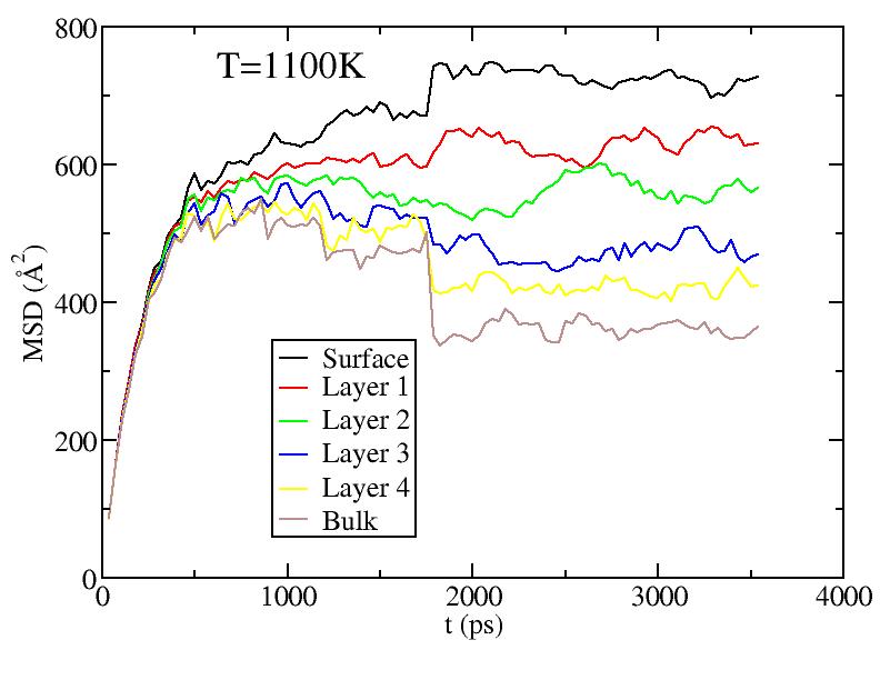
Fitting the MSD vs. t curves above (for T<1100K) to MSD = Dt (i.e. curves pass through origin; Yanting, do I get the coefficient you used correct?) we get the average diffusion constant of atoms in each layer. Diffusion constants here are quite small compared to what they are in the liquid - Yanting, can you use the short time part of the 1100K MSD vs t curve to find D in the liquid just above melting? We will argue below that, below melting, it is not all the atoms that diffuse with the diffusion constant shown below, but rather only a small subset of atoms (those at vertices and edges) that diffuse. Hence, although there is diffusion as low as 600K, until around 900K, most of the atoms on the surface are NOT diffusing, hence there is no surface melting (but this is less clear above 900K).
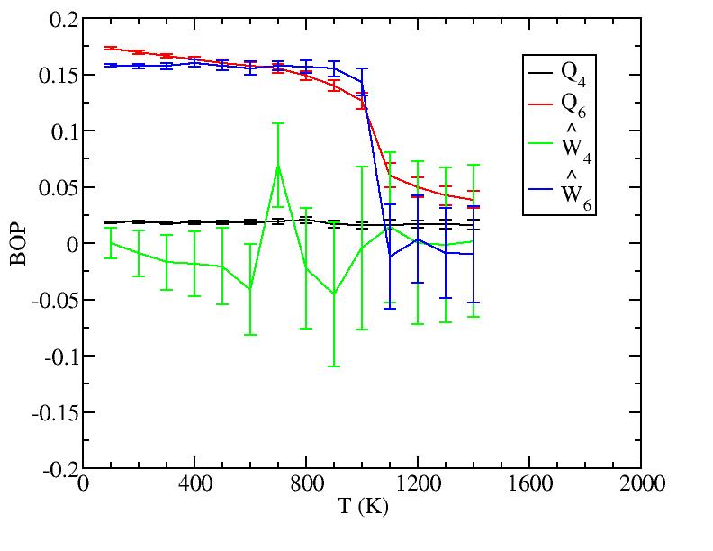
We should add to this graph results from new
simulations at 850K, 950K, 1050K and 1075K that Yanting is doing.
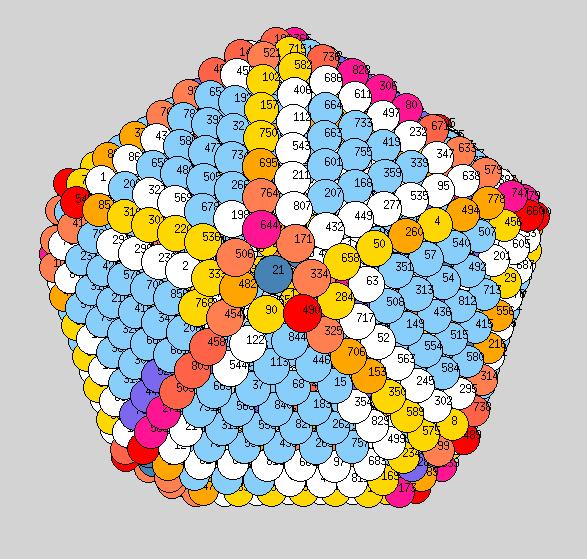
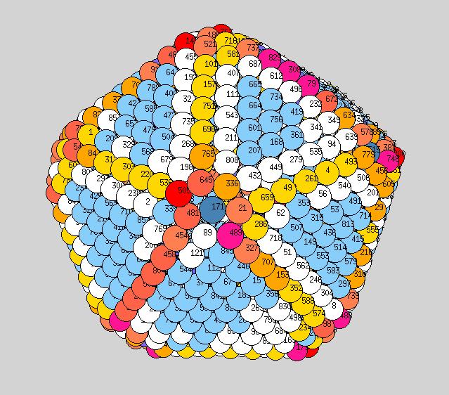
Using the above procedure to define the position of the atoms in the average shape, we then compute the two principle local curvatures of each atom on the surface using Yanting's algorithm The equilibrium shapes, with each atom colored according the the value of its largest of the two principle curvatures, are shown below - scale is blue to red corresponds to small to large curvature.
Observations: at low T we have a very nice ichosohedral fully faceted crystal. It remains like this up to about 600K. Vertices have largest curvature (red), followed by edges (orange or yellow), with facets the smallest curvature (light blue). At 700K we start to see some rounding of the vertices (note: the orientation at 700K is not necessarily the same orientation as shown at 600K, if I remember correctly?). At 900K we see rounded vertices and edges. At 1000K things are now quite rounded, with maybe very small facets still remaining. It will be good to see similar picutres for the new temperatutres 950, 1050, 1075, to see if facets totally dissappear before melting or not.
Yanting, for publication, we should probably take the numbers off the atoms.
400K
600K
700K
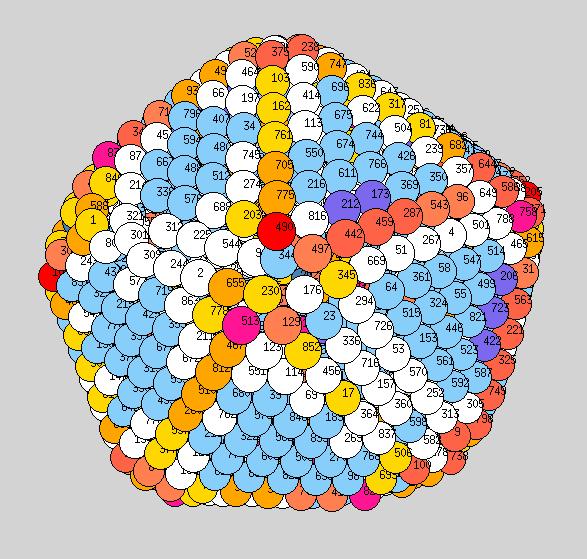
800K
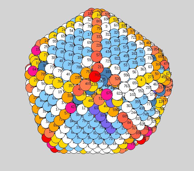
900K
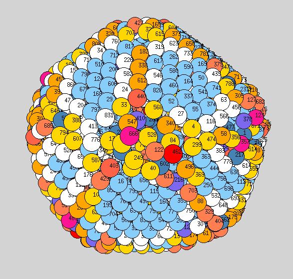
1000K
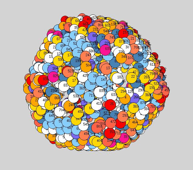
To see this we plot pictures similar to above, ie each atom is located at its average position, however we now adjust the size of each sphere representing a given atom to equal the root mean square distance moved by the atom about its average position, throughout the course of our simulation. Below, for each temperature shown, we plot two such pictures: one averaged over the first 25 stored configurations of the simulation, and the second averaged over 100 stored configurations (Yanting, what simulation time does this correspond to in ps?). The point here is that if a particle is NOT diffusing, the size of its sphere will be the same in both pictures, but if a particle is diffusing, the size of its sphere will roughly double from the first picture to the second (since root mean square distance will grow as square root of time).
Pictures are on Yanting's page, here.
I think these look really nice. It is quite clear that at the lower T<900K, it is only vertices and edges that are diffusing. And even at higher T=900 and 950 one can see facet atoms which are not diffusing.
For a paper, I suggest we show the same temperatures here as we do for the curvature colors pictures in previous section.
Try to make similar pictures for the nanorod, to see if we can correlate what happens here to what happens there. Can one say that the onset of shape change in the nanorod is due to onset of diffusion at vertices and edges?
It the end, it is still unclear how our results are related to the faceting transition. The equilibrium shape in the "Wolf" plot way of thinking has to do with the dependence of surface tension, for in principle an infinite flat plane, on surface orientation. Here, things seem to be goverened by curvature (not included in Wolf construction method) ie by the atoms that have fewest nearest neighbor bonds. On the other hand, even in the Wolf construction point of view, the crystal will round out first at its edges. So I am not sure if there is a connection or if there is not. Also, our cluster is so small that it might not be realistic to use the "infinite size" assumption behind the Wolf construction. Clearly the bulk crystal structure (ichosohedral) we have here is different from that (fcc/hcp) of the rod, so size is obviously important. I will try to think more about this. Any thoughts from others are welcome!