We have already found, in our discussion of combinations and permutations, the probability to flip exactly r heads in N flips of a fair coin. This was

           = 

where  was the number of outcomes which had exactly r heads (number of ways to choose which r of the N coins will be heads), and 2^N was the total number of all possible outcomes of the N flips. Why I chose to rewrite (1/2)^N = (1/2)^r(1/2)^N-r in the last step will become clearer later.

We can also calculate the probability to roll exactly r "6"s in N rolls of a fair die. The number of outcomes that will have exactly r "6"s can be caluculated as  where  is the number of ways to choose which r of the N dice will come up with a "6", and each of the remaining N-r dice can land in anyone of 5 ways (i.e. anything but a "6") thus giving the factor 5^N-r. The total number of all possible outcomes is 6^N, so we can write for the probability to roll exactly r "6"s,

In the above, note that (1/6) is the probability to roll a "6", while (5/6) is the probability not to roll a "6". The factor (1/6)^r(5/6)^N-r is therefore the probability to roll any particular sequence which has exactly r "6"s, and N-r not "6"s. The factor  is the number of ways to choose which r of the N dice will have the "6"s.

The probability for flipping r heads in N coins has exactly the same form as above, if one notes that (1/2) is the probability to flip a head, and (1/2) is the probability to flip a tail (i.e. not a head).

More generally, suppose we have an experiment such that we can classify all the outcomes as one of either two possibilities: "win" or "fail". The probability to win is "p" (where p is any number between 0 and 1) and so the probability to fail is "1-p". What is the probability that in N trials of the experiment one gets r wins?

We argue as above. The probability to get any particular sequence of r wins and N-r fails is p^r(1-p)^N-r. The number of such sequences with r wins is just the number of ways to choose which are the r wining trials out of the N total trials, i.e. . So the total probability to get any one of these sequences with n wins is:

PN(r) = p^r(1-p)^N-r

The above expression is called the binomial distribution.

We want now to get some feeling for how the binomial distribution behaves, as the number of trial N is increases. We consider the specific example of flipping a coin, for which the probability to "win" is p=1/2.

Number of Heads in N flips

How many heads should we expect in N flips of a fair coin? Clearly, for N very large, we expect to get N/2 heads. But we should not always expect exactly N/2; sometimes we might get N/2 +1, and sometimes N/2 -1. We might even get N/2 + 2, or N/2 -2. How far from N/2 would it be reasonable to get? What is the probability that we get exactly r heads in N flips?

From doing this experiment many times on the computer, and recording the fraction of occurrences, we get the following plot for N=10 flips:

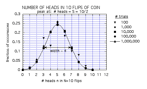
The solid line is the theoretical prediction given by the binomial distribution: 

We see that as the number of trials we perform (i.e. the number of different independent experiments we do of flipping a coin 10 times) increases, the fraction of occurrences of r heads approaches a constant value which agrees well with the predicition P_N(r). As expected, the most likely occurrence, i.e. the value of n where the probability is maximum, is n=N/2=5. However to get exactly n=5 is still only about a 24% chance. The probability to get n=4 or 6 is about 21%, while to get n=3 or 7 is about 12%.

To characterize how far from N/2 we are likely to get, we can define the "width" of the probability distribution as follows. Just look at the value of r for which the probability PN(r) is 1/2 the value of the most likely outcome P_N(N/2). There will be two such values of r, one below N/2 and one above N/2. The difference between them we will call the width. In the above graph, these two values of r are 3 and 7. The width is therefore 4.

There are other ways to define a width. In the text by Ambegaokar he uses the width of the range of r about N/2 such that there is a 99% probability that the outcome will be found within this range of r. I am using the above definition because it is easier to read it off from the graph. Later on we will give a more precise definition for "width". But all these definitions are just meant to give an indication of how far from the most likely outcome N/2, is still a reasonably likely outcome. So for the above graph, we would say that we expect in N=10 trials, to get 5 ± 2 heads in any given trial (the "error" ± 2 comes from the width: 5+2=7, and 5-2=3, giving the width 7-3=4).

Suppose that I now flip the coin N=40 times? On average we expect N/2=20 heads. But how far from this average of 20 would it still be reasonable to get? Naively one might think that if the average goes up by a factor of 4, then the width should also go up by a factor of 4, and so one might expect to get 20 ± 8 heads (giving a width of 16). This turns out not to be correct! Below we show the results of a computer simulation of N=40 flips:

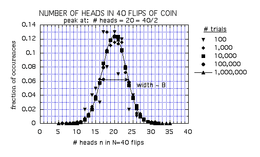
We see that for N=40, the width is only 8. Thus, for N=40 as compared to N=10, the width does not increase by a factor of 4, but only by a factor of 2. So we expect in N=40 flips to see 20 ± 4 heads.
 
 

Similarly, we can consider increasing the number flips by another factor of 4 to N=160. The results of the computer simulation are shown below:

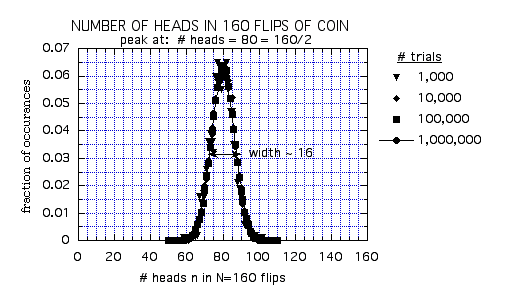
We see that for N=160, the width is 16. Thus, comparing N=160 to N=40, we again see that the most likely outcome increases by a factor of 4, but the width increases by only a factor 2. In N=160 flips we expect to see 80 ± 8 heads.

We summarize the results from these three graphs as follows:

number of    average                   average                                               fractional width    relative error
trials N        number of heads     fraction heads     width        "error"       (width/N)         (error/average)

10                     5                               0.5                 4                2                 4/10 =0.4             2/5 =0.4

40                   20                               0.5                 8                4                 8/40 =0.2           4/20 =0.2

160                 80                               0.5               16                8              16/160=0.1           8/80 =0.1

What conclusions can we make?

1) As N increases, the distributions peak at the same fractional distance from the origin, N/2. This is just a result of the fact that probability to flip a head is 1/2 - hence one expects on average (1/2)N heads.

2) As N increases, the peak in the distribution gets sharper. We can state this more precisely by saying that the fractional width of the distribution, (width/N), gets smaller.

Lets explore the consequences of (2) further. Since the number of all possible outcomes is measured by N (i.e. in N flips we can have anywhere from r=0 to r=N heads as a result), and as the width is a measure of the number of likely outcomes (those whose probability of occurrence is at least half that of the most likely outcome N/2), we see that fractional width is a measure of the ratio of (number of likely outcomes)/(number of possible outcomes). Since the fractional width decreases with increasing N, the number of outcomes for which there is an appreciable probability becomes a smaller and smaller fraction of all possible outcomes as the number of trials increases. As the number of trials increases, we can predict with much greater relative certainty what the outcome must be!

(In the above, we are labeling outcomes by the number of heads found, and not by the specific sequence in which those heads occurred. In N flips of a coin there are in principle 2^N total possible particular sequences of heads and tails that may occur - but these sequences can all be grouped according to the number of heads found in each sequence. To borrow a terminology from physics, we can say that any one of the 2^N particular sequences is a microstate of our system, while labeling the outcomes by the number of heads found in the sequence specifies a macrostate of the system. The microstates are all equally likely to occur, and are unique. A given macrostate consists of many different microstates. The number of microstates that belong to a given macrostate can be different for different macrostates; hence the various macrostates are not equally likely to occur.)

In particular, when N increases by a factor 4, the width increase by only a factor 2 = . This suggest that the width is growing with N as the square root of N, width propto , where "propto" means "proportional to". We can see this by making the following plots. First we plot the width for a given number of trials N, versus N.

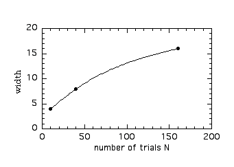
We see that as N increases, the curve bends over - the width grows more slowly than N.

Now we plot the width versus .

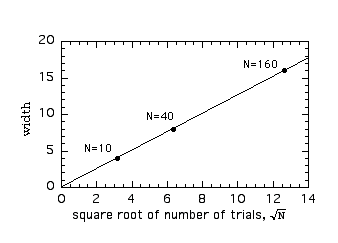
We see that all the data points fall on a straight line. This confirms our conclusion that the width grows like .

We can make this relation more precise by measuring the slope of the line in the above graph. The slope is just the difference in height along the vertical axis divided by the difference in distance along the horizontal axis, for any two points on the line. For the above line we can take as the two points (, 4) and (0,0) (when we write a point on a graph as a pair of numbers (x,y), the first number is the position on the horizontal axis, the second number is the position on the vertical axis). The slope is then (4-0)/(-0) = 4/ = 1.265. Since the above line goes through the point (0,0), we can write the equation for this line as:

width = (slope)  ()  = 1.265.

The fractional width then decreases with increasing N as:

   =     = .

Similarly, since the error is 1/2 the width, we can write

error = 0.6325 ,

and for the relative error,

.

This result, which we will see is quite general, is of very great importance when we come to apply these probabilistic ideas to understand the behavior of physical systems. It will mean that for systems which consist of very large numbers of seemingly random elements (for example the many atoms of a gas), because the number of elements is so large (for a gas it is typically of order 10²³ atoms!) we can predict with virtual certainty the outcome of measurements of certain average quantities.

Observation (2) can also be understood by going back to our beginning definition of what we meant by the term "probability". Probability was defined as follows: If the probability to flip a head is 1/2, then for a very large number of trials N we expect to find (1/2)N heads. Now in any given experiment of N flips, we know that we will not in general get exactly N heads. We will get sometimes more, sometimes less. From the above table we see that if we flip N=10 times, we should expect to get 5±2 heads. If we define as our "measurement" of the probability to get one head in one flip, the number of heads divided by the number of flips, we are likely to measure in any one experiment of 10 flips a probability (5±2)/10 = 1/2 ± 1/5 to flip a head. The relative error in our measurement of the probability to flip a head is likely to be as big as ("error"/average) = 2/5 = 0.4 or 40% off!

Now for N=40 flips, we expect to get 20±4 heads. A measurement of the probability to flip a head is then (20±4)/40 = 1/2 ± 1/10. The relative error in our measurement is likely to be as big as 4/20 = 1/5 = 0.2 or 20% off. Similarly, for N=160 flips, we are likely to get 80±8 heads. Our measured probability is then (80±8)/160 = 1/2 ± 1/20. The relative error in our measurement is likely to be as big as 8/80 = 1/10 = 0.1 or 10% off.

So we see that as we increase the number of trials N, the accuracy with which we can measure correctly the probability to get one head in one flip increases. This is directly a consequence of the fact that the relative width of the distribution decreases with increasing N. The fact that the accuracy of our measurement increases (i.e. relative error decreases) with increasing N, is essential for our definition of probability to be meaningful in the first place. If the relative error did not decrease with increasing N, we could never measure accurately the probability to flip a head, no matter how many times we flipped our coin! By understanding how to compute the width of the probability distribution, and seeing how precisely the relative width decreases with increasing N, we will be able to quantify what we mean by "a very large number" of trials, in our definition of probability. That is, we will be able to specify exactly how large N should be in order that the likely error in the measurement of the probability will be a given small number.