We now return to investigate the connection between the standard deviation and the "width" we defined earlier. In the process of doing this, we will come upon a very important property of the binomial distribution, and understand the deeper meaning of the standard deviation.
First we plot below the binomial probability distributions for three different cases:
(1) the probability for r wins in N=4 trials, when
the probability for one win is p=1/2
(2) the probability for r wins in N=5 trials, when
the probability for one win is p=1/3
(3) the probability for r wins in N=11 trials, when
the probability for one win is p=1/10
In each case, the probability distribution plotted is obtained from our general formula
![]()
using the appropriate values of N and p, for r=0, 1, ...,N.
I have chosen these three cases because they all
have a standard deviation of approximately unity. We can see this as follows.
Using our earlier results that ![]() and
and ![]() , we have
for the three cases
, we have
for the three cases
(1) ![]()
(2) ![]()
(3) ![]()
Using our earlier results for the mean, µ1=p, and µN=N µN, we find the mean of the three cases are:
(1) µ=4![]() =2
=2
(2) µ =5![]() =1.667
=1.667
(3) µ=11![]() =1.1.
=1.1.
The graphs of the three probability distributions are:
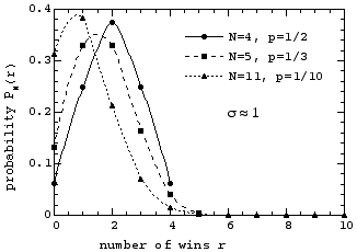
Remember, the probability distribution is measured at integer values of r only, and is shown in the graph by the circle, square, and triangle symbols. The lines connecting these points are only guides to the eye to help distinguish the three different cases from each other.
Note the following about the three curves above. For case (1) with p=1/2, the curve is completely symmetric about its mean µ = 2; this is a consequence of the fact that for p = 1/2 the probability to win is the same as the probability to lose. For case (2) however, with µ =1.667, and more clearly so for case (3) with µ=1.1, the curves are not symmetric about their mean; this is a consequence of the fact that for any p ≠ 1/2, the probability to win is different from the probability to lose.
To see that the shapes of the three curves are indeed different, we now translate the curves so that the horizontal origin will lie at the mean value for each of the three distributions; that is, we plot the probability distributions PN(r) versus the distance from their mean values r - µ.
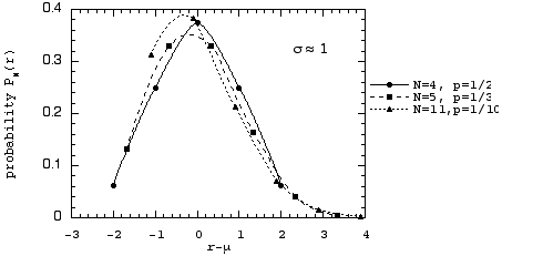
In these plots, the lack of symmetry about the mean for cases (2) and (3) can be more clearly seen. That the curves for the three cases have different shapes should not be surprising; they represent, after all, three completely different binomial distributions with different values of p and N.
However, consider now what happens when we increase
N in each case, so that all the distributions have a larger value of the
standard deviation, ![]() ≈
2. We choose the cases:
≈
2. We choose the cases:
(1) N=16, p=1/2 with mean µ =
16![]() = 8 and standard
deviation
= 8 and standard
deviation ![]()
(2) N=18, p=1/3 with mean µ =
18![]() = 6 and standard
deviation
= 6 and standard
deviation ![]()
(3) N=45, p=1/10 with mean µ =
45![]() = 4.5 and
= 4.5 and ![]()
We first plot these distributions versus the number of wins r:
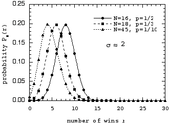
Note that the curves now all appear symmetrical about their mean, with a characteristic "bell" shape. This becomes more obvious when we plot the distributions versus the distance from the mean, r - µ.
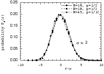
The peaks all lie essentially at the mean value, and the distributions are much more nearly symmetrical about the mean. But something more interesting than these observations is to be seen! The points for the three difference cases now all fall on very close to a single curve!
We can again increase N in each of the three cases
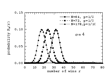
so that now the standard deviations are all ![]() ≈ 4. We choose the cases:
≈ 4. We choose the cases:
(1) N=64, p=1/2, with
µ =
64![]() = 32 and
= 32 and ![]()
(2) N=72, p=1/3, with µ =
72![]() = 24 and
= 24 and ![]()
(3) N=178, p=1/10, with µ =
178![]() = 17.8 and
= 17.8 and ![]() .
.
We first plot these distributions versus the number of wins r:
We now replot these probability distributions versus the distance from their mean, r-µ:
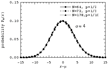
Even more so than in the previous case with ![]() ≈ 2, we see that for
≈ 2, we see that for ![]() ≈ 4, all the points lie on one single curve.
≈ 4, all the points lie on one single curve.
What we have just observed empirically is that as
N increases, the binomial distribution approaches a universal curve
which is characterized by just two quantities: its mean µ
and its standard deviation ![]() .
This universal curve is known as the normal probability distribution,
or also the Gaussian probability distribution.
.
This universal curve is known as the normal probability distribution,
or also the Gaussian probability distribution.
Thus for N sufficiently large, different binomial
distributions, with different values of N and p, but with the same ![]() ,
will all have the exact identical shape, only with peaks centered at their
respective means µ=Np. Hence when we replot
these distributions shifting their peaks to the origin, or equivalently
plotting them versus r - µ, they all fall
on one universal curve.
,
will all have the exact identical shape, only with peaks centered at their
respective means µ=Np. Hence when we replot
these distributions shifting their peaks to the origin, or equivalently
plotting them versus r - µ, they all fall
on one universal curve.
That the shape of the large N binomial distribution
depends only on ![]() ,
and not on the detailed parameters of the distribution N and p, is a surprising
result that is extremely important! To prove this result mathematically,
and write the equation which describes the normal distribution,
is beyond the scope of this course. For now we just point out that the
properties of this normal distribution have been very extensively studied.
Among them are the facts that:
,
and not on the detailed parameters of the distribution N and p, is a surprising
result that is extremely important! To prove this result mathematically,
and write the equation which describes the normal distribution,
is beyond the scope of this course. For now we just point out that the
properties of this normal distribution have been very extensively studied.
Among them are the facts that:
(1) The two points µ + ![]() and
µ
-
and
µ
- ![]() locate
the two values of r where the probability has decreased from its value
at the peak µ by a factor of
locate
the two values of r where the probability has decreased from its value
at the peak µ by a factor of ![]() = 0.7071, i.e. P(µ +
= 0.7071, i.e. P(µ + ![]() )=
P(µ
-
)=
P(µ
- ![]() )
= 0.7071P(µ). Thus 2
)
= 0.7071P(µ). Thus 2![]() is comparable to our empirically defined "width" which measured the distance
between the values of n for which P(n) = 0.5P(µ).
Since
is comparable to our empirically defined "width" which measured the distance
between the values of n for which P(n) = 0.5P(µ).
Since ![]() measures
a smaller decrease from P(µ) than the "width"
did, 2
measures
a smaller decrease from P(µ) than the "width"
did, 2![]() is somewhat
smaller than the "width".
is somewhat
smaller than the "width".
(2) If one adds up the probabilities for all the
values of r between µ + ![]() and µ -
and µ - ![]() ,
this adds up to 0.6827. Thus the outcome of the experiment has a 68% chance
to lie within one standard deviation of the mean. Similarly, if one adds
up the probabilities for all values of r between µ + 2
,
this adds up to 0.6827. Thus the outcome of the experiment has a 68% chance
to lie within one standard deviation of the mean. Similarly, if one adds
up the probabilities for all values of r between µ + 2![]() and µ - 2
and µ - 2![]() ,
this adds up to 0.9545. Thus the outcome of the experiment has a 95% chance
to lie within two standard deviations of the mean. Similarly, the outcome
has a 99% chance to lie within 2.6 standard deviations of the mean. One
can make a table of the probability to lie within an interval specified
by so many standard deviations (or fractions of a standard deviation) from
the mean:
,
this adds up to 0.9545. Thus the outcome of the experiment has a 95% chance
to lie within two standard deviations of the mean. Similarly, the outcome
has a 99% chance to lie within 2.6 standard deviations of the mean. One
can make a table of the probability to lie within an interval specified
by so many standard deviations (or fractions of a standard deviation) from
the mean:
Standard Deviations Probability
0.1 0.0797
0.5 0.3829
1.0 0.6827
1.5 0.8664
2.0 0.9545
2.5 0.9876
3.0 0.9973
3.5 0.9995
4.0 0.9999
Thus virtually all the probability of the normal distribution is concentrated within a few standard deviations of the mean. This is why the standard deviation is such an important parameter for describing a probability distribution.
How big must N be for the binomial distribution to
be well approximated by the normal distribution? As a rough rule of thumb,
it must be true that the standard deviation ![]() should be very much less than the mean µ.
Even when this holds true, the normal distribution will be a good approximation
for the binomial distribution only in the range of several standard deviations
about the mean. The approximation will not be so good in the tails very
far from the mean. The size of the range about the mean for which the normal
is a good approximation increases as N increases.
should be very much less than the mean µ.
Even when this holds true, the normal distribution will be a good approximation
for the binomial distribution only in the range of several standard deviations
about the mean. The approximation will not be so good in the tails very
far from the mean. The size of the range about the mean for which the normal
is a good approximation increases as N increases.
What we have seen above regarding the large N behavior
of the binomial distribution, is actually a much more general feature of
probability distributions. When we consider the number of wins r in N trials
of an experiment, we can view the number of wins r as being the sum of
the number of wins in each individual trial. The number of wins in each
individual trial is of course either 1 or 0. As we add more and more trials,
the probability for the sum of the results (that is the binomial distribution)
approaches the normal distribution. One can now imagine another type of
"elementary" experiment in which there are more than two possible outcomes.
As an example, the role of a die can have 6 outcomes, which we can label
by the number on the face which lands on top. Suppose we roll the die N
times, and we want the probability distribution for the sum of the faces
which land on top. It turns out that for N sufficiently large, this is
also a normal distribution! Virtually anytime one adds the results of many
trials of an "elementary" experiment, then regardless of the probability
distribution for the outcomes of the "elementary" experiment (provided
it is not too pathological), if N is sufficiently large the result will
be well approximated by a normal distribution with mean µN
=
Nµ1, and
standard deviation ![]() N
=
N
= ![]()
![]() 1,
where µ1
and
1,
where µ1
and ![]() 1
are the mean and the standard deviation of the "elementary" experiment.
This result is known as the Central Limit Theorem. The general proof
of this theorem is beyond the scope of this course, however if you go back
to our proof of the results µN
=
Nµ1 and
1
are the mean and the standard deviation of the "elementary" experiment.
This result is known as the Central Limit Theorem. The general proof
of this theorem is beyond the scope of this course, however if you go back
to our proof of the results µN
=
Nµ1 and ![]() N
=
N
= ![]()
![]() 1
for the binomial distribution, you will see that they hold quite generally
for the sum of any N "elementary" experiments (in the proof, we never had
to explicitly use the binomial form for the distribution PN(n);
hence the proof works for the sums of any arbitrary distribution P(n)).
1
for the binomial distribution, you will see that they hold quite generally
for the sum of any N "elementary" experiments (in the proof, we never had
to explicitly use the binomial form for the distribution PN(n);
hence the proof works for the sums of any arbitrary distribution P(n)).