Basic Introduction to Python
This is a very basic introduction to Python. It is not exhaustive, but is meant to give you a starting point.
This notebook was written for PHY 403 by Segev BenZvi, University of Rochester, (Spring 2016).
It is based on a similar (longer) Python guide written by Kyle Jero (UW-Madison) for the IceCube Programming Bootcamp in June 2015, and includes elements from older guides by Jakob van Santen and Nathan Whitehorn.
What is Python?
Python is an imperative, interpreted programming language with strong dynamic typing.
- Imperative: programs are built around one or more subroutines known as "functions" and "classes"
- Interpreted: program instructions are executed on the fly rather than being pre-compiled into machine code
- Dynamic Typing: data types of variables (
int,float,string, etc.) are determined on the fly as the program runs - Strong Typing: converting a variable from one type to another (e.g.,
inttostring) is not always done automatically
Python offers fast and flexible development and can be used to glue together many different analysis packages which have "Python bindings."
As a rule, Python programs are slower than compiled programs written in Fortran, C, and C++. But it's a much more forgiving programming language.
Why Use Python?
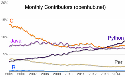
Python is one of the most popular scripting languages in the world, with a huge community of users and support on all major platforms (Windows, OS X, Linux).
Pretty much every time I've run into a problem programming in Python, I've found a solution after a couple of minutes of searching on google or stackoverflow.com!
Key Third-Party Packages
Must-Haves
- NumPy: random number generation, transcendental functions, vectorized math, linear algebra.
- SciPy: statistical tests, special functions, numerical integration, curve fitting and minimization.
- Matplotlib: plotting: xy plots, error bars, contour plots, histograms, etc.
- IPython: an interactive python shell, which can be used to run Mathematica-style analysis notebooks.
Worth Using
- SciKits: data analysis add-ons to SciPy, including machine learning algorithms.
- Pandas: functions and classes for specialized data analysis.
- AstroPy: statistical methods useful for time series analysis and data reduction in astronomy.
- Emcee: great implementation of Markov Chain Monte Carlo; nice to combine with the package Corner.
Specialized Bindings
Many C and C++ packages used in high energy physics come with bindings to Python. For example, the ROOT package distributed by CERN can be run completely from Python.
Online Tools
If you don't want to install all these packages on your own computer, you can create a free account at wakari.io.
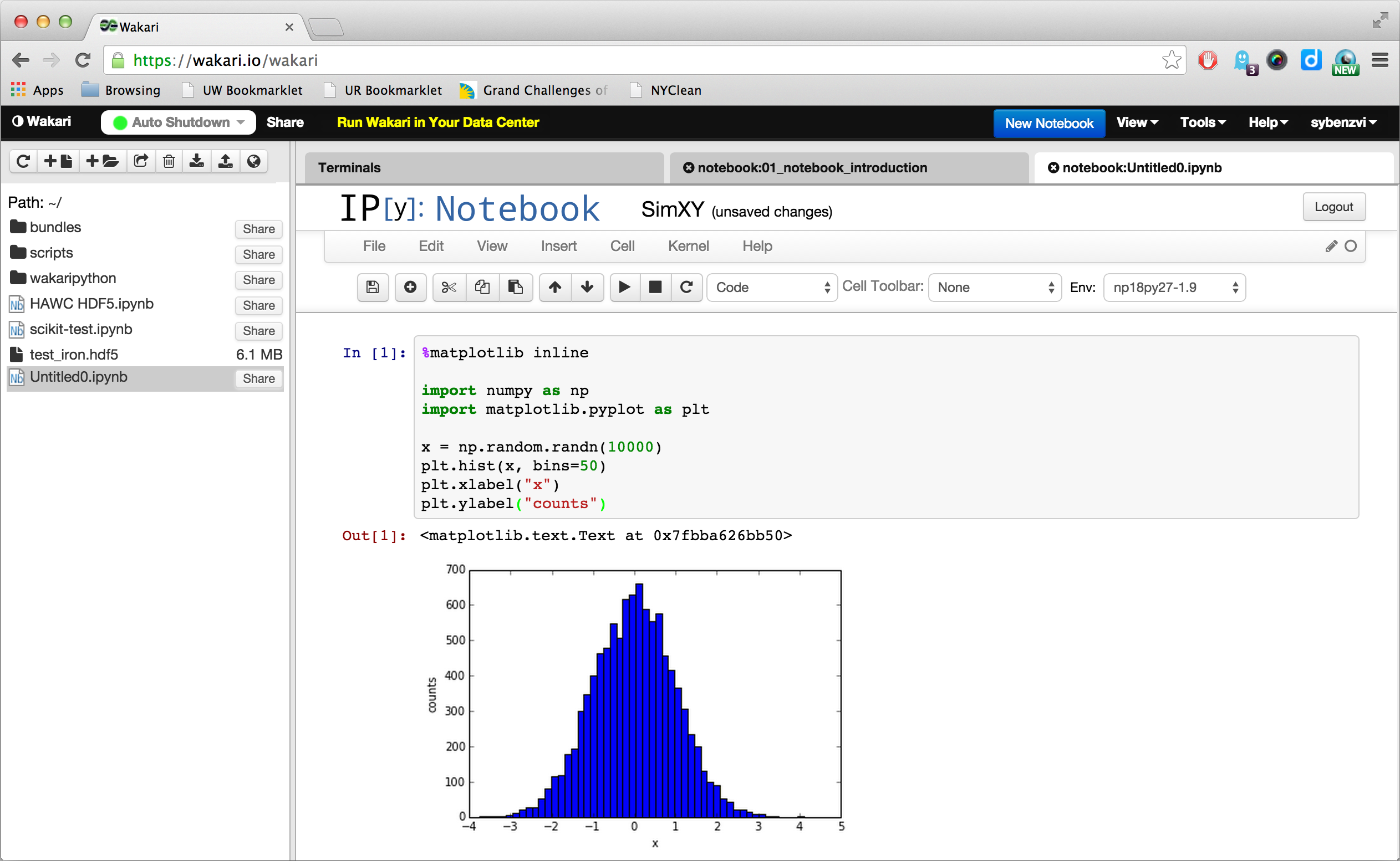
Wakari gives you access to ipython notebooks running on remote servers. Recent versions of SciPy, NumPy, and Matplotlib are provided.
Programming Basics
We will go through the following topics, and then do some simple exercises.
- Arithmetic Operators
- Variables and Lists
- Conditional Statements
- Loops (
forandwhile) - Functions
- Importing Modules
Arithmetic Operators
Addition
1+2
Subtraction
4 - 1
Multiplication
3*8
Division
50 / 2
1 / 2
Note: in Python 2, division of two integers is always floor division. In Python 3, 1/2 automatically evaluates to the floating point number 0.5. To use floor division in Python 3, you'll have to run 1 // 2.
1.0000000 / 2
float(1) / 2
Modulo/Remainder
30 % 4
3.14159265359 % 1.
Exponentiation
2**4
Variables
Variables are extremely useful for storing values and using them later. One can declare a variable to contain the output of any variable, function call, etc. However, variable names must follow certain rules:
- Variable names must start with a letter (upper or lower case) or underscore
- Variable names may contain only letters, numbers, and underscores _
The following names are reserved keywords in Python and cannot be used as variable names:
and del from not whileas elif global or withassert else if pass yieldbreak except import printclass exec in raisecontinue finally is returndef for lambda try
x = 5 + 6
This time nothing printed out because the output of the expression was stored in the variable x. To see the value we have to call the print function:
print(x)
Alternatively, just call x and the notebook will evaluate it and dump the value to the output:
x
Recall that we don't have to explicitly declare what type something is in python, something that is not true in many other languages, we simply have to name our variable and specify what we want it to store. However, it is still nice to know the types of things sometimes and learn what types python has available for our use.
print(type(x))
y = 2
print(type(x/y))
z = 1.
print(type(z/y))
h = 'Hello'
print(type(h))
s = " "
w = "World!"

print(h + s + w)
apostrophes="They're "
quotes='"hypothetically" '
saying=apostrophes + quotes + "good for you to know."

print(saying)
C-style formatted printing is also allowed:
p = "Pi"
print("%s = %.3f" % (p, 3.14159265359))
Lists
Imagine that we are storing the heights of people or the results of a random process. We could imagine taking and making a new variable for each piece of information but this becomes convoluted very quickly. In instances like this it is best to store the collection of information together in one place. In python this collection is called a list and can be defined by enclosing data separated by commas in square brackets. A empty list can also be specified by square brackets with nothing between them and filled later in the program.
blanklist=[]
blanklist
alist=[1,2,3]
print(alist)
print(type(alist))
Notice that the type of our list is list and no mention of the data type it contains is made. This is because python does not fuss about what type of thing is in a list or even mixing of types in lists. If you have worked with nearly any other language this is different then you are used to since the type of your list must be homogeneous.
blist=[1, "two", 3.0]
blist
print(type(blist))
You can check the current length of a list by calling the len function with the list as the argument:
len(blist)
In addition, you can add objects to the list or remove them from the list in several ways:
blist.append("4")
blist
blist.insert(0, "0")
blist
blist.extend([5,6])
print(blist)
print(len(blist))
blist.append(7)
blist
blist = blist*2
blist
blist.remove("4")
blist
blist.remove('4')
blist
List Element Access
Individual elements (or ranges of elements) in the list can be accessed using the square bracket operators [ ]. For example:
print(blist[0])
print(blist[4])
print(blist[-1])
print(blist[-2])
print(blist[-3])
blist[0:4]
print(blist)   # list slicing example:
blist[0:6:2]   # sytax: start, stop, stride
This is an example of a slice, where we grab a subset of the list and also decide to step through the list by skipping every other element. The syntax is
listname[start:stop:stride]
Note that if start and stop are left blank, the full list is used in the slice by default.
blist[::2]
print(blist[::-1])   # An easy way to reverse the order of elements
print(blist)
A simple built-in function that is used a lot is the range function. It is not a list but returns one so we will discuss it here briefly. The syntax of the function is range(starting number, ending number, step size ). All three function arguments are required to be integers with the ending number not being included in the list. Additionally the step size does not have to be specified, and if it is not the value is assumed to be 1.
range(0,10)
range(0,10,2)
Conditional Statements
Conditionals are useful for altering the flow of control in your programs. For example, you can execute blocks of code (or skip them entirely) if certain conditions are met.
Conditions are created using if/elif/else blocks.
For those of you familiar with C, C++, Java, and similar languages, you are probably used to code blocks being marked off with curly braces: { }
In Python braces are not used. Code blocks are indented, and the Python interpreter decides what's in a block depending on the indentation. Good practice (for readability) is to use 4 spaces per indentation. The IPython notebook will automatically handle the indentation for you.
x = 55

if x > 10:
    print("x > 10")
elif x > 5:
    print("x > 5")
else:
    print("x <= 5")
isEven = (x % 2 == 0)    # Store a boolean value

if not isEven:
    print("x is odd")
else:
    print("x is even")
Comparison Operators
There are several predefined operators used to make boolean comparisons in Python. They are similar to operators used in C, C++, and Java:
== ... test for equality
!= ... test for not equal
> ... greater than
>= ... greater than or equal to
< ... less than
<= ... less than or equal to
Combining Boolean Values
Following the usual rules of boolean algebra, boolean values can be negated or combined in several ways:
Logical AND
You can combine two boolean variables using the operator && or the keyword and:
print("x  y  |  x && y")
print("---------------")

for x in [True, False]:
    for y in [True, False]:
        print("%d  %d  |  %d" % (x, y, x and y))
x = 10
if x > 2 and x < 20:
    print(x)
if x < 2 and x > 20:
    print(x)
Logical OR
You can also combine two boolean variables using the operator || or the keyword or:
print("x  y  |  x || y")
print("---------------")

for x in [True, False]:
    for y in [True, False]:
        print("%d  %d  |  %d" % (x, y, x or y))
x = 10
if x > 2 or x < 0:
    print(x)
if x < 2 or x > 20:
    print(x)
Logical NOT
It's possible to negate a boolean expression using the keyword not:
print("x  | not x")
print("----------")
for x in [True, False]:
    print("%d  |  %d" % (x, not x))
A more complex truth table demonstrating the duality
$\overline{AB} = \overline{A}+\overline{B}$:
print("A  B  |  A and B  |  !(A and B)  | !A or !B")
print("-------------------------------------------")
for A in [True, False]:
    for B in [True, False]:
        print("%d  %d  |  %-7d  |  %-12d|  %d" %
              (A, B, A and B, not (A and B), not A or not B))
Loops
Loops are useful for executing blocks of code as long as a logical condition is satisfied.
Once the loop condition is no longer satisfied, the flow of control is returned to the main body of the program. Note that infinite loops, a serious runtime bug where the loop condition never evaluates to False, are allowed, so you have to be careful.
While Loop
The while loop evaluates until a condition is false. Note that loops can be nested inside each other, and can also contain nested conditional statements.
i = 0
while i < 10:         # Loop condition: i < 10
    i += 1            # Increment the value of i
    if i % 2 == 0:    # Print i if it's even
        print(i)
For Loop
The for loop provides the same basic functionality as the while loop, but allows for a simpler syntax in certain cases.
For example, if we wanted to access all the elements inside a list one by one, we could write a while loop with a variable index i and access the list elements as listname[i], incrementing i until it's the same size as the length of the list.
However, the for loop lets us avoid the need to declare an index variable. For example:
for x in range(1,11):    # Loop through a list of values [1..10]
    if x % 2 == 0:       # Print the list value if it's even
        print(x)
for i, x in enumerate(['a', 'b', 'c', 'd', 'e']):
    print("%d  %s" % (i+1, x))
If we are interested in building lists we can start from a blank list and append things to it in a for loop or use a list comprehension which combines for loops and list creation into line. The syntax is a set of square brackets that contains formula and a for loop.
squaredrange = [e**2 for e in range(1,11)]

print(squaredrange)
You can also loop through two lists simultaneously using the zip function:
mylist  = range(1,11)
mylist2 = [e**2 for e in mylist]

for x, y in zip(mylist, mylist2):
    print("%2d %4d" % (x, y))
Functions
Functions are subroutines that accept some input and produce zero or more outputs. They are typically used to define common tasks in a program.
Rule of thumb: if you find that you are copying a piece of code over and over inside your script, it should probably go into a function.
Example: Rounding
The following function will round integers to the nearest 10:
def round_int(x):
    return 10 * ((x + 5)/10)

for x in range(2, 50, 5):
    print("%5d %5d" % (x, round_int(x)))
In-Class Exercise
With the small amount we've gone through, you can already write reasonably sophisticated programs. For example, we can write a loop that generates the Fibonacci sequence.
Just to remind you, the Fibonacci sequence is the list of numbers
1, 1, 2, 3, 5, 8, 13, 21, 34, 55, ...
It is defined by the linear homogeneous recurrence relation
$F_{n} = F_{n-1} + F_{n-2}$, where $F_0=F_1=1$.
The exercise is:
- Write a Python function that generate $F_n$ given $n$.
- Use your function to generate the first 100 numbers in the Fibonacci sequence.
# Easy implementation: recursive function

def fib(n):
    """Generate term n of the Fibonacci sequence"""
    if n <= 1:
        # if n==0 or n==1: return 1
        return 1
    else:
        return fib(n-1) + fib(n-2)
for n in range(0, 35):
    Fn = fib(n)
    print("%3d%25d" % (n, Fn))
This function will work just fine for small n. Unfortunately, the recursive calls to fib cause the function call stack to grow rapidly with n. When n gets sufficiently large, you may hit the Python call stack limit. At that point your program will crash.
Here is a more efficient approach that does not require recursion:
def fibBetter(n):
    """Generate the Fibonacci series at position n"""
    a, b = 0, 1
    while n > 0:                 # build up the series from n=0
        a, b, n = b, a+b, n-1    # store results in loop variables
    return b
for n in range(0, 100):
    Fn = fibBetter(n)
    print("%3d%25d" % (n, Fn))
Accessing Functions Beyond the Built-In Functions
If we want to use libraries and modules not defined within the built-in functionality of python we have to import them. There are a number of ways to do this.
import numpy, scipy
This imports the module numpy and the module scipy, and creates a reference to that modules in the current namespace. After you’ve run this statement, you can use numpy.name and scipy.name to refer to constants, functions, and classes defined in module numpy and scipy.
numpy.pi
from numpy import *
This imports the module numpy, and creates references in the current namespace to all public objects defined by that module (that is, everything that doesn’t have a name starting with “_”).
Or in other words, after you’ve run this statement, you can simply use a plain name to refer to things defined in module numpy. Here, numpy itself is not defined, so numpy.name doesn’t work. If name was already defined, it is replaced by the new version. Also, if name in numpy is changed to point to some other object, your module won’t notice.
pi
from scipy import special

print(special.erf(0),
      special.erf(1),
      special.erf(2))
This imports the module scipy, and creates references in the current namespace functions in the submodule special. We then make 3 function calls to the Error Function erf.
import numpy as np
np.pi
np.arange(0,8) # acts like the range function, but return a numpy array
np.arange(0,8, 0.1) # unlike builtin range, you can use non-integer stride
This imports numpy but assigns the name of the module to np so that you can type np rather than numpy when you want to access variables and functions defined inside the module.
NumPy Tips and Tricks
NumPy is optimized for numerical work. The array type inside of the module behaves a lot like a list, but it is vectorized so that you can apply arithmetic operations and other functions to the array without having to loop through it.
For example, when we wanted to square every element inside a python list we used a list comprehension:
mylist = range(1,11)
[x**2 for x in mylist]
This isn't that hard, but the syntax is a little ugly and we do have to explicitly loop through the list. In contrast, to square all the elements in the NumPy array you just apply the operator to the array variable itself:
myarray = np.arange(1,11)
myarray**2
Evenly Spaced Numbers
NumPy provides two functions to give evenly spaced numbers on linear or logarithmic scales.
np.linspace(1, 10, 21) # gives 21 evenly spaced numbers in [1..10]
np.logspace(1, 6, 6)     # gives 6 logarithmically spaced numbers
                         # between 1e1=10 and 1e6=1000000
np.logspace(1, 6, 6, base=2) # same as above, but base-2 logarithm
Slicing Arrays with Boolean Masks
An extremely useful feature in NumPy is the ability to create a "mask" array which can select values satisfying a logical condition:
x = np.arange(0, 8)      # [0, 1, 2, 3, 4, 5, 6, 7]
y = 3*x                  # [0, 3, 6, 9, 12, 15, 18, 21]

c = x < 3
print(c)
print(x[c])
print(y[c])
print(y[x >= 3])
c = (x<3) | (x>5)         # Combine cuts with bitwise OR or AND
print(y[c])
This is the type of selection used all the time in data analysis.
File Input/Output
Standard Python has functions to read basic text and binary files from disk.
However, for numerical analysis your files will usually be nicely formatted into numerical columns separated by spaces, commas, etc. For reading such files, NumPy has a nice function called genfromtxt:
# Load data from file into a multidimensional array
data = np.genfromtxt("data.txt")

x = data[:,0]   # x is the first column (numbering starts @ 0)
y = data[:,1]   # y is the second column

print(x)
print(y)
Plotting with Matplotlib
Matplotlib is used to plot data and can be used to produce the usual xy scatter plots, contour plots, histograms, etc. that you're used to making for all basic data analyses.
I strongly recommend that you go to the Matplotlib website and check out the huge plot gallery. This is the easiest way to learn how to make a particular kind of plot.
Note: when you want to plot something in an IPython notebook, put the magic line
%matplotlib inline
before you import the matplotlib module. This will ensure that your plots appear inside the notebook. Otherwise the plots will pop open in another window, which can be annoying.
%matplotlib inline

import matplotlib.pyplot as plt
plt.plot(x, y, "k.")
plt.xlabel("x [arb. units]")
plt.ylabel("y [arb. units]")
plt.title("Some XY data")

Here is an example of how to change the default formatting of the text in your plot. Also note how LaTeX is supported!
import matplotlib as mpl
mpl.rc("font", family="serif", size=16)

plt.plot(x, y, "k.")
plt.xlabel(r"$\sin({x)}$ [arb. units]")
plt.ylabel(r"$\zeta(y)$ [arb. units]")
plt.title("Some XY data")

Using NumPy and Matplotlib Together
Here we create some fake data with NumPy and plot it, including a legend.
x = x=np.linspace(-np.pi, np.pi, 1000,endpoint=True)
c = np.cos(x)
s = np.sin(x)

plt.plot(x,c,label="Cosine",color="r",linestyle="--",linewidth=2)
plt.plot(x,s,label="Sine",color="b",linestyle="-.",linewidth=2)
plt.xlabel("$x$",fontsize=14)
plt.xlim(-np.pi,np.pi)

# Override default ticks and labels
xticks = [-np.pi, -0.5*np.pi, 0, 0.5*np.pi, np.pi]
labels = ["$-\pi$", "$-\pi/2$", "$0$", "$\pi/2$", "$\pi$"]
plt.xticks(xticks, labels)

plt.ylabel("$y$",fontsize=14)
plt.ylim(-1,1)
plt.legend(fontsize=14, loc="best", numpoints=1)

Help Manual and Inspection
When running interactive sessions, you can use the built-in help function to view module and function documentation.
For example, here is how to view the internal documentation for the built-in function that calculates the greatest common divisor of two numbers:
from fractions import gcd

help(gcd)
The inspect module is nice if you actually want to look at the source code of a function. Just import inspect and call the getsource function for the code you want to see:
from inspect import getsource

print(getsource(gcd))