Numerical quantum mechanics (one-dimensional)
This little program solves the eigenstate problem H|Psi> = E|Psi> numerically for an arbitrary hamiltonian H. Just plug in your potential V and seconds later take a peek at the eigenstates and eigenvalues. I'm sure all of this could be done in smarter ways, but I like that all the machinery is exposed. The only matlab trickery we use is matrix multiplication.
Tobin Fricke tfricke@ligo.caltech.edu 2009-02-12
Contents
Numerical setup
First we have to define a grid on which we'll compute our eigenfunctions
n = 100;                   % number of points
x = linspace(-4, 4, n)';

% How many eigenstates do we want to find?
N_eigenstates_to_find = 10;
eigenvalue_accuracy = 1e-5;

% Now we have to define the derivative operator.  We do this by following
% the definition of the derivative as lim (h->0) of (f(x+h)-f(x))/h and
% just setting h to delta x.
h = (x(2)-x(1));  % assume a uniform grid
D = (- diag(ones(1,n-1),-1) + diag(ones(1,n-1),1)) / (2 * h); % the derivative!
D(n,1) = 1/h; % periodic boundary conditions

Dsquared = (diag(ones(1,n-1),1) - 2*diag(ones(1,n)) + diag(ones(1,n-1), -1))/h^2;
PHYSICS
% Define some useful quantum mechanical operators
p = i * D;                       % the momentum operator

% Definte the potential
V = (abs(x) > 2)*1000;              % square-well potential

% Define the hamiltonian
H = -Dsquared + diag(V);               % the Hamiltonian
Find some eigenvalues and eigenstates
Here we use the 'iteration method' to find the eigenvalues and eigenstates of H. Because the iteration method finds the greatest eigenvalue, and we want the least eigenvalue, we solve for the eigenvalues of inv(H) instead of (H). See: http://nibot-lab.livejournal.com/85743.html
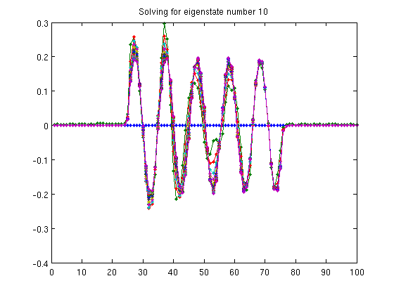
% There are surely better algorithms to find the eigenvectors.  This was
% the first that came to mind.

% Pre-allocate space for our lists of eigenvectors and eigenvalues
vs      = zeros(n,N_eigenstates_to_find) * NaN;
lambdas = zeros(N_eigenstates_to_find)   * NaN;

lambda_previous = NaN;
lambda          = NaN;

Hinv = inv(H);  % compute H^(-1)

for jj=1:N_eigenstates_to_find
    fprintf('Solving for the %0.0fth eigenstate...', jj);
    % Start with a random unit vector
    v = rand(size(x));
    v = v / sqrt(v'*v);
    % Here we just initialize some variables
    lambda_previous = NaN;
    lambda = NaN;
    N_iterations = 0;
    hold off;
    % Iterate until the eigenvalue converges to some value
    while not(abs(lambda - lambda_previous)/(lambda + lambda_previous) < eigenvalue_accuracy),
        % Remember the previous estimate of the eigenvalue
        lambda_previous = lambda;
        % Apply the map v <-- A v
        v = Hinv * v;
        % We can estimate the eigenvalue by looking at how the length
        % changed
        lambda = 1/sqrt(v'*v);
        v = v*lambda;
        % Subtract the projections of this vector onto all previously found
        % eigenvectors
        for kk=1:(jj-1)
            v = v - vs(:,kk) * vs(:,kk)' * v;
        end
        % Just for fun, count how many times we iterate
        N_iterations = N_iterations + 1;
        % Watch the convergence in action...
        plot(v, '.-');
        title(sprintf('Solving for eigenstate number %0.0f', jj));
        drawnow;
        hold all
    end
    hold off;
    % Make sure this is a unit vector before we store it
    v = v / sqrt(v' * v);
    % Store the newly found eigenvector and eigenvalue
    vs(:, jj) = v;
    lambdas(jj) = lambda;
    % Announce our success:
    fprintf(' found in %0.0f iterations, with eigenvalue %g\n', ...
        N_iterations, lambda);
end
Solving for the 1th eigenstate... found in 4 iterations, with eigenvalue 0.57482
Solving for the 2th eigenstate... found in 9 iterations, with eigenvalue 2.29716
Solving for the 3th eigenstate... found in 7 iterations, with eigenvalue 5.16061
Solving for the 4th eigenstate... found in 14 iterations, with eigenvalue 9.15465
Solving for the 5th eigenstate... found in 21 iterations, with eigenvalue 14.2643
Solving for the 6th eigenstate... found in 18 iterations, with eigenvalue 20.4709
Solving for the 7th eigenstate... found in 11 iterations, with eigenvalue 27.751
Solving for the 8th eigenstate... found in 29 iterations, with eigenvalue 36.0788
Solving for the 9th eigenstate... found in 26 iterations, with eigenvalue 45.4211
Solving for the 10th eigenstate... found in 19 iterations, with eigenvalue 55.7453
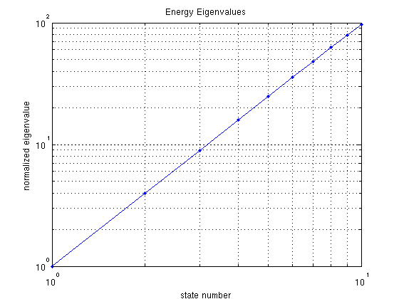
Plot the energy levels found
loglog(lambdas./lambdas(1), '.-');
xlabel('state number');
ylabel('normalized eigenvalue');
title('Energy Eigenvalues');
grid on;
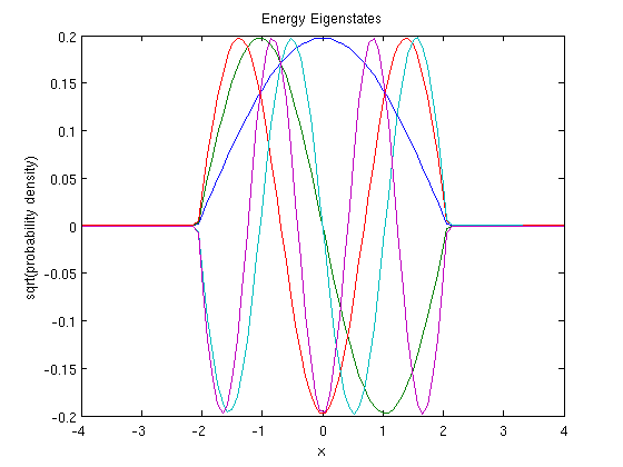
Plot the eigenstates
hold off;
for ii=1:5;%size(vs,2)
    plot(x, (vs(:,ii)));
    hold all;
end
hold off;
title('Energy Eigenstates');
xlabel('x');
ylabel('sqrt(probability density)');