Contents

Set up procesing parameters

array station locations

x = [4000 0; 0 4000; 0 0; 2000 0; 0 2000; 1000 100];

% Change the LIGO coordinate system (in which the X arm is in the x
% direction and the Y arm is in the y direction to one in which North is
% "up" (positive y direction).  The paper arXiv:gr-qc/0403046 says that the
% X arm has compass bearing 324 degrees (northwest).

theta = (324.0 - 360 - 90)*pi/180;
R = [cos(theta), sin(theta); -sin(theta), cos(theta)];
x = (R * x')';

% kgrid parameters

kpoints = 40;  % number of sample points in each direction
kmax = 3/2000; % maximum wavenumber in each direction

Read the data

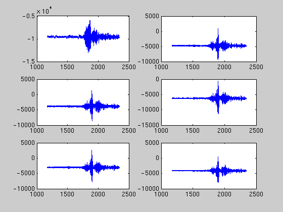
data = dlmread('quake-wf.txt');
data = data';
samprate = 256;

% Crop the data
data = data(:,3e5:6e5);

% Separate out the time channel
times = data(1,:);
data(1,:) = [];

Plot the timeseries

for i=1:6,
    subplot(3,2,i);
    plot(times,data(i,:));
end

Plot some spectra

fdata = abs(fft(data'))';
%faxis =

Decimate the timeseries

decimation = 10;
dsamprate = ceil(samprate/decimation);
[rows cols] = size(data);
ddata=zeros(rows,ceil(cols/decimation));

% Apply the decimation to each row.

for r=1:rows,
    ddata(r,:) = decimate(data(r,:),decimation);
end

Investigate pairwise cross-correlation

for i=1:rows,
    for j=1:rows,
        [c,lags]=xcorr(ddata(i,:),ddata(j,:),500,'unbiased');
        [bestc,index]=max(c);
        bestlag(i,j) = lags(index(1));
    end
end
bestlag,

bestlag =

     0   -83   -87  -104   -85  -118
    83     0    -7   -24    -4   -29
    87     7     0   -17     3   -21
   104    24    17     0    20    -4
    85     4    -3   -20     0   -24
   118    29    21     4    24     0

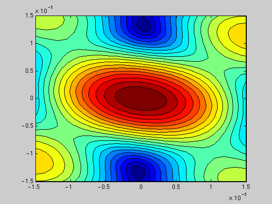
Build the k-grid

k = (((-kpoints+1)/2):((kpoints-1)/2)) * 2 * kmax / (kpoints -1);
kgrid = zeros(kpoints, kpoints, 2);
[kgrid(:,:,1), kgrid(:,:,2)] = meshgrid(k,k);

Compute the array's antenna response function

rgrid = zeros(kpoints,kpoints);
omega = 2 * pi * (dsamprate/2); % consider the nyquist frequency
zoom = 100;
for i=1:kpoints,
    for j=1:kpoints,
        rgrid(i,j) = abs(sum(exp(sqrt(-1)*omega* squeeze(kgrid(i,j,:)/zoom)' * x')));
    end
end
subplot(1,1,1);
contourf(kgrid(:,:,1)/zoom,kgrid(:,:,2)/zoom,rgrid,20);

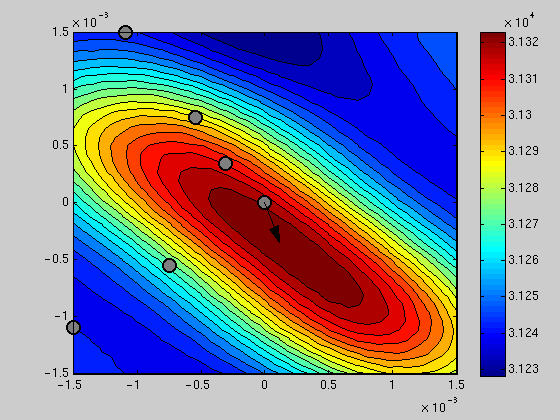
Do the beamforming

% The beamformer is really slow.  Use of the profiler indicates that nearly
% all of the time is spent copying data.  To write a fast beamformer, I
% think we'd have to write it in C.

pgrid = beamform(kgrid, x, ddata, dsamprate);

Find the best beam power

[R,C] = ind2sub(size(pgrid),find(pgrid ==max(max(pgrid))));;
kbest = squeeze(kgrid(R,C,:));

% Compute the corresponding azimuth (compass bearing)
azimuth = 90 - atan2(kbest(2),kbest(1))*180/pi

azimuth =

  161.5651

Plot the beam power versus k-vector

hold off;
contourf(kgrid(:,:,1),kgrid(:,:,2),pgrid,20);
hold on;
colorbar;

% Superimpose a diagram of the sensor array for directional reference
xmax = max(max(x));
plot(x(:,1)*kmax/xmax,x(:,2)*kmax/xmax,'ko','LineWidth',2,'MarkerSize',12,'MarkerEdgeColor','k','MarkerFaceColor',[0.5 0.5 0.5])

% Draw an arrow indicating the best k-vector
arrow([0 0],kbest);
hold off;

% Another idea for estimating the incoming wavevector was to create a
% weighted sum of all k-vectors on the grid, each weighted by the beam
% power it produced.  However, this doesn't seem to produce a good answer.

kvote = [sum(sum(pgrid .* squeeze(kgrid(:,:,1)))) , ...
         sum(sum(pgrid .* squeeze(kgrid(:,:,2)))) ] / sum(sum(pgrid));

Published with MATLAB® 7.1