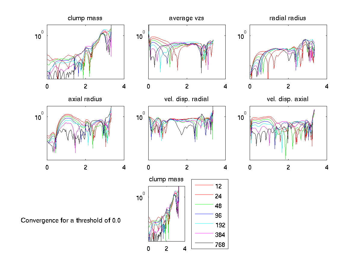
Global quantities
These are plots of our six quantities versus time. Each line is a different resolution. For the most part, there is decent "convergence" up to about t=1.
The linked movie shows the effect of varying the tracer threshold from 0.0 (any tracer amount) to 1.0 (100% tracer only). Some of the quantities (such as mass) change noticeably with varying threshold, as expected.

Convergence (relative error)
These are plots of the quantities' convergence (i.e., relative error) against 1536, versus time. Each line is a different resolution. What is important about these plots is the wide variability of the error over time. In the literature it is typical to report relative errors at a single (arbitrary?) moment in time. It is clear from these plots that doing so could lead to misleading results.
The linked movie shows the effect of varying the tracer threshold from 0.0 (any tracer amount) to 1.0 (100% tracer only). In contrast to the movie above, the relative error seems robust with respect to varying this threshold.
The y-range is [1e-4 : 1e1]. These are log(y) plots.
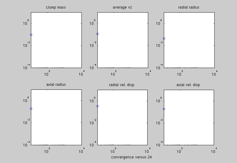
Time-averaged relative error
These are plots of relative error against 1536 averaged over the entire simulation, versus resolution. Each dot is a different resolution. This shows that, when the error is averaged over the entire simulation, no particular convergence across resolutions is noted.
The linked movie shows the effect of comparing successively lower-resolution runs (described in more detail in the next paragraphs).
Effect of sampling window on time-averaged relative error: starting from t=0.
These are plots of relative error versus sampling window size. The question is, what is the effect of the period over which you average the relative error? To clarify: each point on a line gives the value of the relative error averaged from t=0 to that point in time. So the righthand most point (x=3.5) shows the result from averaging over the entire simulation time.
The linked movie shows the effect of resolution. The first frame compares 1536 to all, the second frame compares 768 to all but 1536, etc. In most cases, the closest resolution (768 vs 1536, 384 vs 768, etc.) has similar relative error. Hence, relative error alone can be misleading. That is, small relative error between resolutions says nothing about whether the simulation itself is "correct." The relative error between 24 and 48 may be of the same order as the relative error between 768 and 1536—but no one thinks the 48 cells/rclump simulation has sufficient resolution. Indeed, in some cases (look at radial radius), reducing the resolution improves the relative errors.
Looking at relative error alone also doesn't make sense if your highest resolution case is capable of resolving fluid dynamics which the others are not. This is exactly what we're expecting in this case. What if the radial radius or radial velocity dispersion is much different in the 1536 case because we're finally able to sufficiently resolve the "boundary layer"? This might appear to be divergence, not convergence, according to a plot of relative error.
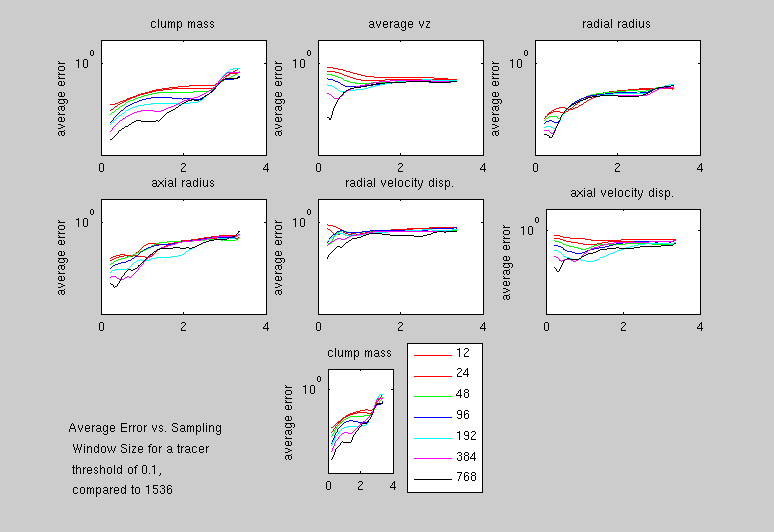
(Ignore the 7th plot; I couldn't get MATLAB to give me a floating legend so I included another plot just to attach the legend to.)
Effect of sampling window on time-averaged relative error: starting from t=t0.
These are the same plots as in the image above. The movie which is linked, however, shows the effect of moving the sampling window from t~0 to t~tend. So, as the movie progresses, each point on the line gives the result of averaging from the start of the line up to that point in time. The shapes of the curves are relatively robust to the start time, indicating that the error is more a function of the time of the simulation than the location of the sampling window.
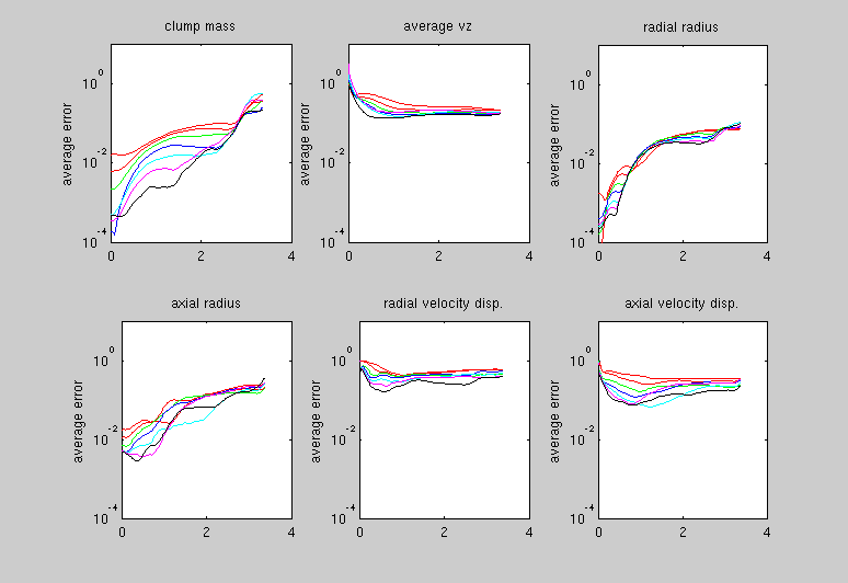
(Ignore the 7th plot; I couldn't get MATLAB to give me a floating legend so I included another plot just to attach the legend to.)
Effect of sampling window on time-averaged relative error: let's look at more complicated graphs
The above line plots are slices of the 2D parameter space of sampling window tstart vs sampling window tend. Contour plots of this space are given below. The important point is that flat regions in the plot are regions where the relative error is not changing much versus the sampling window. Hence, if we are going to do some kind of temporal sampling, we should probably focus on these regions.
Note however that in most cases as you go up in resolution, the size of this region decreases


Here are the same plots, but versus 768 instead of 1536. Note that in most cases the relative errors are smaller.


Effect of sampling window on time-averaged relative error: standard deviation over time of relative error
To be done.
One would hope that with increasing resolution both the average relative error and the standard deviation of the relative error with respect to time would decrease. However, considering the "shrinking flat region" behavior noted above, this may not be the case.