
Most recent blog posts
Testing Outflow Feedback
Posted on: September 18, 2016
A rotating protostellar core collapses to form a star and outflow. This movie comes from initial exploratory simulations using newly incorporated feedback routines in AstroBEAR. The outflow seen here is based on the two-component sub-grid model of Federrath et al (2014).
Reorientation of oblique MHD shocks
Posted on: August 18, 2016
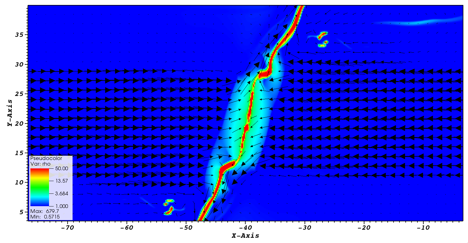
An unexpected result from our 3D, high-res, oblique colliding flows simulations (Fogerty et al. 2016) was the large-scale realignment of the collision layer, which reoriented post-shock gas normal to the upstream magnetic field and velocity vectors. Not only was this effect interesting from a purely MHD fluid dynamics perspective, but also from a star formation perspective: prestellar filaments are widely believed to arise from turbulent compressive motions in the ISM, and have been observed to lie perpendicular to environmental magnetic fields.
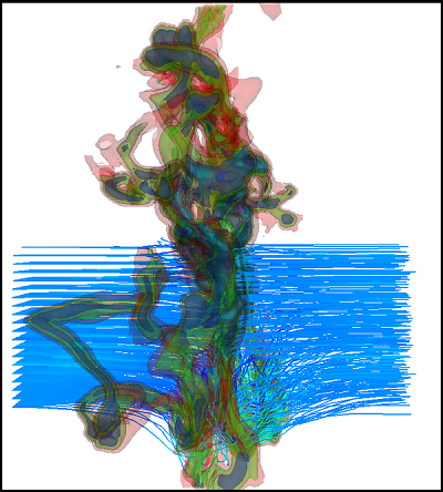
To explore the driving mechanism of reorientation, we performed a set of idealized 2D simulations. Here is a snapshot from one of the runs, which was initialized with a *highly* oblique collision interface of 60°. This run had an initially weak magnetic field (a few µG) that was aligned along the flows and was uniform everywhere within the simulation domain. The flows were marginally supersonic (M=1.5) and each had an inflow speed of 11 km s-1. The initial number density of the gas was n=1 cm-3. As can be seen from the plot, post-shock gas reorients normal to the upstream flows (velocity vectors are overlaid, and are scaled by magnitude).
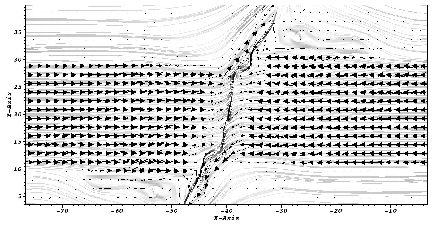
The next plot shows the corresponding magnetic field structure. Note that field lines are distorted both by passage through the shocks, as well as collision with post-shock ejecta. The color of the field lines indicate the local magnetic field strength (field lines increase in strength from light gray to black), and thus, illustrate regions of field amplification.
 Additional reorientation movies can be found under the 'Movies' tab on the menu bar above, as well as on youtube. For further reading, see Fogerty et al. 2016, which is currently under review.
Radiating sink particle
Posted on: February 20, 2016
 movie
movie
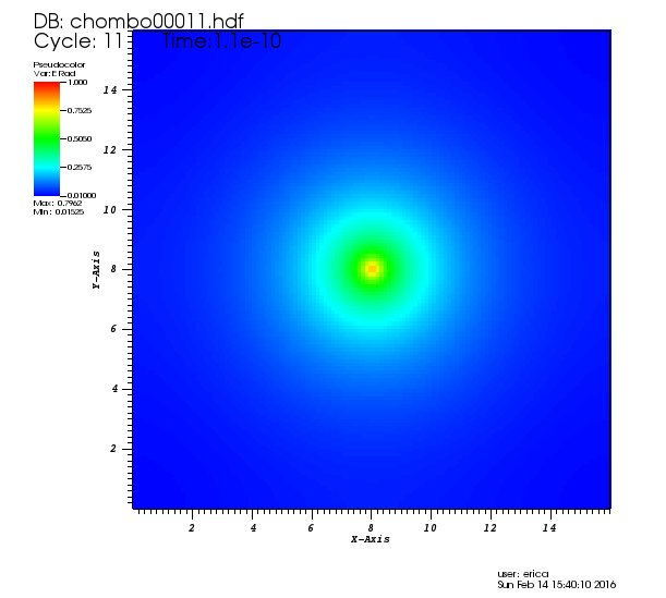
Excited to have a sink particle on the grid that is 'radiating'. This movie comes from an initial test simulation of the newly completed radiative feedback module in AstroBEAR. As you can see, the sink is producing a nice, spherical radiation field -- given by the radiative energy, 'Erad'.
Choosing the accretion luminosity for radiative feedback
Posted on: January 26, 2016
The amount of energy released as heat when a particle passes through the accretion shocks at the surface of a star is related to the particle's kinetic energy at that instant, which can be calculated most easily for a particle that starts at rest from infinity. Equating the particle's rest energy at infinity (=0) with its energy at the surface of the star shows,
For a stream of parcels, we can ask how much energy is released per unit time? This is given by the time-derivative of the above equation (i.e. the accretion luminosity):
Now, material is only accreted by a sink from the immediately surrounding zones. So to track the energy released from this accretion per unit time, one could imagine calculating the right hand side of the previous equation in the code, for gas within an 'accretion volume'. To do so would implicitly assume the gas:
- Started from rest at infinity, and freely falls onto the surface of the star
- Only feels the gravitational pull of the star
Given gas in the accretion volume has not traveled from infinity in free-fall to the sink surface, one might be inclined to instead use,
which describes the luminosity due to gas falling in from a distance r away (instead of infinity). However, as the following plots show, using this equation for different values of the kinetic energy at r, ke(r), where ke(r)=1/2 mv^2^(r) in the above equation, does not produce wildly differing accretion energies until you move close-in to the surface of the star. In fact, in all but the most extreme cases, the degree of error is negligible (<1%), even at a distance of 1/100,000 of a parsec (i.e. much less than a typical cell size). At that distance, it doesn't matter whether the gas parcel is starting from rest, moving slowly (less than freefall speed), or moving fast (up to 10x freefall speed), the accretion energy that parcel will release at the stellar surface ''is the same''. This provides a clear example of how most of the energy gained from gravitational infall occurs in the final legs of the journey.
Therefore under most circumstances, using the simpler form for the accretion luminosity should be a *great* approximation. In this prescription, m-dot will be the accreted mass per timestep, M will be the mass of the sink each timestep, and R will be an input variable to the code the user can set. By default, R will be a solar radius. This accretion energy will be smoothed over a kernel of cells surrounding the sink every time step, which will then diffuse through the rest of the grid via flux-limited diffusion.
Interestingly...
An alternative to this approach would be using the left hand side of the equation, the accreted kinetic energy per timestep, which would be very nice: it wouldn't rely on an ''estimate'' of the accretion luminosity, but rather, it would use the accreted kinetic energy itself. However, we do not track accreted kinetic energy onto the sink. This is because of the 'sub-grid' nature of the sink: we do not have distance information within the sink particle, therefore, have no way of knowing how much kinetic energy makes its way onto the star. Other processes during infall could convert the kinetic energy into heat, etc. That is to say, energy is not conserved during accretion events. Therefore, we are stuck with an approximation for the accretion luminosity.
Bones, tombs, and planets
Posted on: Oct. 10, 2015
Astronomy on tap is a public outreach event that hosts popular science talks by local astronomers. Thanks to Jen Connelly for inviting me to tell the story of Newgrange, an astronomical temple that was built in 3000 B.C.E. These ruins captured my imagination after recently visiting them on a trip to Ireland. My talk is about prehistoric human behavior and technology, constructing the temple, bones and other artifacts that were found in the temple, and fascinating explanations for why it was built. If you can't make my talk, you can check out the slides here.
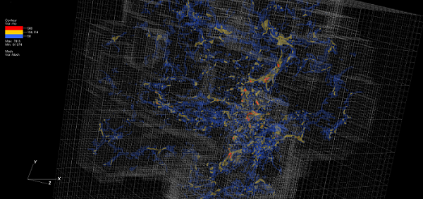
Density isocontours of a molecular cloud, embedded within a high-res, AMR mesh
Posted on: April 16, 2015
Article on our Colliding Flows sims in Rochester's Research Magazine
Posted on: November 21, 2014
Rochester's Center for Integrated Research Computing (CIRC) recently opened the Vista Collaboratory. The collaboratory houses a dedicated 'visualization wall', comprised of tiled, floor-to-ceiling, high-definition screens. The wall is powered by in-house supercomputing nodes, which facilitates intensive data processing and visualization, on the fly. In short, it's awesome.
To celebrate its opening, CIRC sponsored a contest for data visualization. This would showcase the powerful capabilities
of the Collaboratory to the University and wider NY state research community. Our simulations of molecular cloud formation won 1st place, and the University's
news team wrote up a nice piece on our work, have a read here.
Exploring 2D, Approximate Riemann Solvers
Posted on August 3rd, 2013
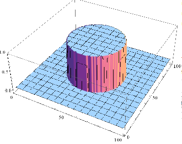
Here is a simple hydrodynamical simulation of a cylindrical explosion, using a 2D Riemann Solver I wrote based on the Godunov method and operator splitting. This is part of a larger project I have been working on to explore Eulerian numerical fluid dynamics. The above image shows the initial conditions of the test problem: the x,y plane gives position, and density is plotted along z. Click on the link to watch the cylindrical shock wave propagate outward into the ambient medium. A more detailed write up can be found here.
Testing self-gravity in AstroBEAR
Posted on: June 23, 2013
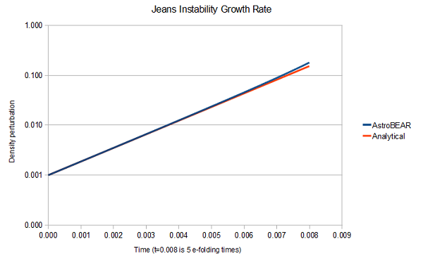
As a test of the self-gravity algorithm in AstroBEAR, I have been working on comparing the analytical growth rate of a Jeans unstable mode to a numerical simulation of an unstable Jeans mode (in 1D), using AstroBEAR. As this plot shows, AstroBEAR closely matches the analytical growth rate over many e-folding times. This result, as well as a detailed explanation of the self-gravity algorithm, will be in the appendix of our upcoming paper on Bonnor-Ebert sphere collapse (Kaminski et al. 2014). Additionally, a write-up on this test can be found here.