The main motivation of the project is the speedup associated with Adaptive Mesh Refinement (AMR) over Fixed Grid codes. This speedup grants us access to what would otherwise be prohibitively expensive calculations of uninvestigated physics. The relevant example is the three dimensional, multiple-Fourier-mode, ablatively supported Rayleigh-Taylor instability.
AstroBEAR benefits from both AMR and parallelization. The graph below illustrates these gains over a fixed grid, single-processor code:
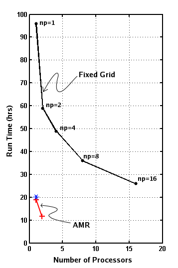
We found that doing AMR in the usual manner -- refining spatial discontinuities in the fluid variables -- leads to spurious features at the interface. If you instead refine a region around the interface, you maintain much of the AMR benefit, without spurious effects. The problem that generated the above plot received a 5-fold speedup from AMR.
Region-criteria AMR and Fixed Grid Return the Same (Correct) Growth
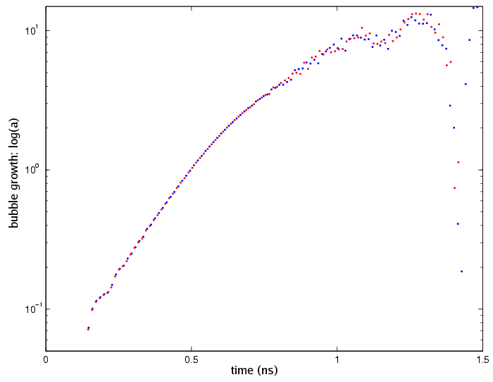
The following graph illustrates that fixed grid (blue) and AMR (red) evolve identically, into the nonlinear growth regime.
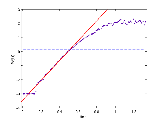
A fit to the growth rate returns a value of γ with uncertainty of a few percent which brackets the analytic value for this setup.
| γanalytic | = (ATkg)1/2 | = (0.9048 (2&pi/10μm) (100μm/ns²))1/2 |
| ≈ 7.54 ns-1 | ||
| and γsim | = 7.1±0.7 ns-1 , |
where AT = (ρH-ρL) / (ρH+ρL) is the Atwood number.
The Linear System Solver Functioned As Expected
The newly-created linear system solver was applied to the equation,
with the coefficient K being a constant, this reduces to
where α = K/ρcv is the thermal diffusivity. The linear solver performed in this case,
| K = 5e-2 | K = 0. | No Linear Solve |
|---|---|---|
 |
 |
 |
Heat conduction with an exponent above 0.3 (K∝T0.3) was found to be too extreme for the solver. (Recall that an exponent of 2.5 was ultimately desired.)
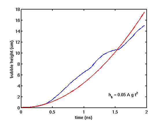
2D Multimode, Classic RT Growth Rate was Confirmed
Instead of perturbing the unstable interface with a single wavemode, one can perturb with a spectrum of modes. This "multimode" seeding will affect the growth and the morphology of the instability.
The above is an region-AMR simulation with 4 levels total (256x1024 maximum resolution). Mode numbers n=1, 2, 4, 8, 16, 32 corresponding to cells-per-wavelength of 256, 128, 64, 32, 16, 8 were seeded. The perturbation was in velocity; the only difference between this simulation and our previous single-mode simulations was the multimode seed (all other parameters were the same).
Theory suggests the value of the bubble height with respect to time will depend on a bubble growth constant αb,
The value of αb is expected to be
| αb | = 0.05–0.06 | for 2D |
| αb | ≈ 0.03 | for 3D |
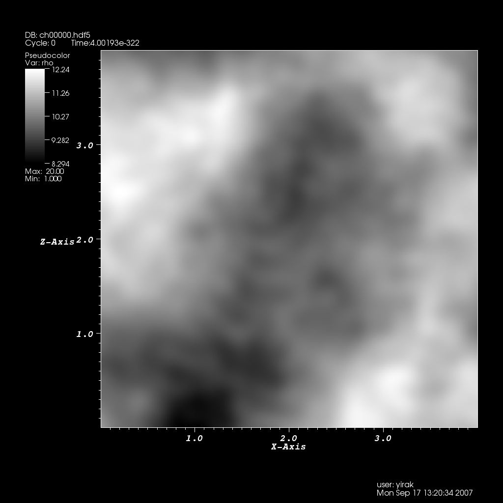
3D Multimode, Classic RT Initialization was Shown to be Consistent with Published Work
Published studies of the 3D multimode RT typically perturb the interface itself rather than seed a velocity perturbation. The wave numbers were chosen with random orientation and a magnitude proportional to k-2. (additional details)
Below is a cross-cut in the x-z plane ("vertical" is in the y-direction) at the interface. The wavemodes to be seeded is user-controlled; below are two examples.
|
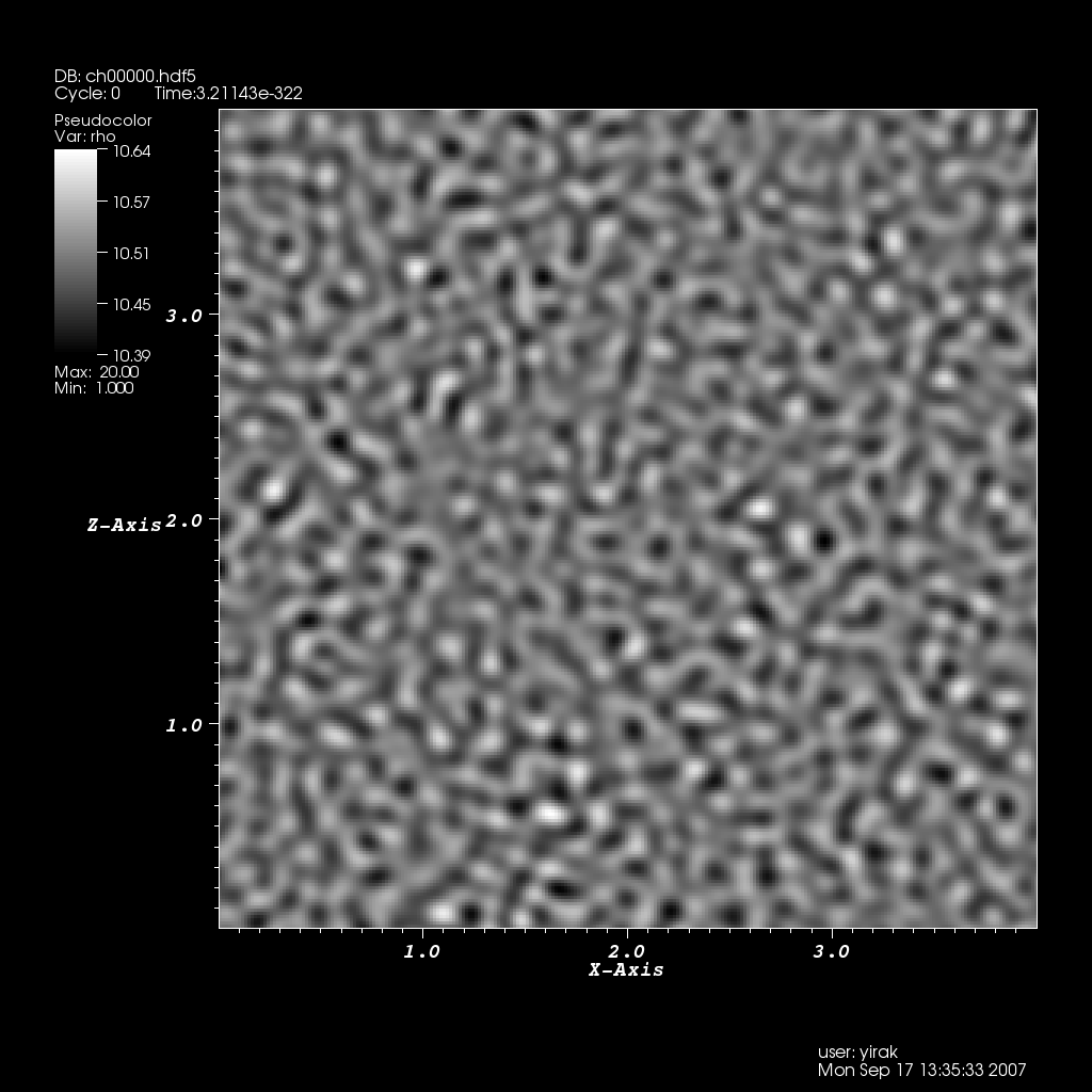
|
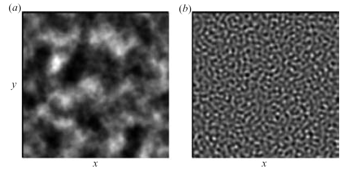
For comparison, below is a published figure from Ramaprabhu et al. 2005. Note that the figure on the left does not depict the same initialization as the above left figure (though it is straightforward to produce such a corresponding image).
At the time, difficulties were encountered getting the simulation to run.